Le pipeline pas à pas et en images#
Nous présentons ici un exemple simple et complet reposant sur une collection de traces simulées à partir d’un réseau. Le réseau est un extrait de la BDTOPO situé sur un versant de montagne en face de la ville de Chamonix, il représente un cas non complexe de tronçons.
Ce pipeline est exécuté en une seule itération.
Import des librairies#
Les deux librairies socles : tracklib et footprint2graph
Pour visualiser les résultats : matplotlib
[1]:
import os
import sys

import matplotlib.pyplot as plt

# Ajout dans la variable PATH du système du chemin où est installée la librairie tracklib
module_path = os.path.abspath(os.path.join('../../../../tracklib'))
if module_path not in sys.path:
    sys.path.append(module_path)
# Alias pour tracklib
import tracklib as tkl

# Ajout dans la variable PATH du système du chemin où est installée la librairie footprint2graph
module_path = os.path.abspath(os.path.join('../../..'))
if module_path not in sys.path:
    sys.path.append(module_path)
Import des données : réseau puis traces simulées#
[2]:
# WKT;link_id;source;target;direction;wkt_source;wkt_target
fmt = tkl.NetworkFormat({
       "pos_edge_id": 1,
       "pos_source": 2,
       "pos_target": 3,
       "pos_wkt": 0,
       "srid": "ENU",
       "separator": ";",
       "header": 1})
netpath = os.path.abspath(os.path.join('../../../data/network2.csv'))
network = tkl.NetworkReader.readFromFile(netpath, fmt, verbose=False)

plt.figure(figsize=(8, 6))
network.plot('k-', '', 'g-', 'r-', 0.5, plt)

print ('Number of edges=', len(network.EDGES))
print ('Number of nodes=', len(network.NODES))
print ('')
Number of edges= 7
Number of nodes= 8
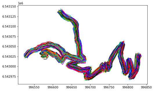
[3]:
tkl.stochastics.seed(333)
#
noiser = tkl.NoiseProcess(amps=2.5, kernels=tkl.ExponentialKernel(80))

# generate simulated trajectories from the network
collection = tkl.generateTracksOnNetwork(network, N=1000, p_round_trip=0.05, p_cplx_trip=0.10, resolution=1, noiser=noiser)

# add 3 attributes
for idx, track in enumerate(collection):
    track.createAnalyticalFeature('TID', idx+1)

#
plt.figure(figsize=(8, 5))
collection.plot(append=plt)
100% (1000 of 1000) |####################| Elapsed Time: 0:00:18 Time: 0:00:180001
------------------------------------------------------------
877 (87.7 %) tracks generated on network
------------------------------------------------------------
Dossier de stockage des résultats#
[4]:
from footprint2graph import prepareEnv, setupEnv, logEnv

RESPATH = r'/home/md_vandamme/7_LIB/footprint2graph/test/resultjn/'

import os
import shutil

# Suppression des répertoires
prepareEnv(RESPATH)

# Création des répertoires
iteration_index = 1
setupEnv(RESPATH, iteration_index)

# Log environment information
logEnv(RESPATH)

#  On définit un format pour le stockage des traces modifiées dans le pipeline
fmt = tkl.TrackFormat({'ext': 'CSV',
                       'srid': 'ENU',
                       'id_E': 1, 'id_N': 0, 'id_U': 3, 'id_T': 2,
                       'time_fmt': '2D/2M/4Y 2h:2m:2s',
                       'separator': ';',
                       'header': 0,
                       'cmt': '#',
                       'read_all': True})

pipeline_idx = 1
Step 1 : segmentation and resampling#
[5]:
from footprint2graph import segmentation_resample

# Paramètre : Nombre de points minimum pour un morceau de trace au moment du découpage
#             si le nombre n'est pas atteint, le morceau de trace est oublié
NB_OBS_MIN           = 10

# Paramètre : Distance en mètres entre 2 points, si supérieure au seuil on coupe la trace
DIST_MAX_2OBS        = 50


RESAMPLE_SIZE_GRID = 1
RESAMPLE_SIZE_FUSION = 5

# =============================================================================
#  On définit un format pour le stockage des traces modifiées dans le pipeline

segmentation_resample(RESPATH, collection, fmt, NB_OBS_MIN, DIST_MAX_2OBS,
                    RESAMPLE_SIZE_GRID, RESAMPLE_SIZE_FUSION)
Starting segmentation and resampling...
Starting segmentation ...
     500 / 877
    Number of tracks after segmentation: 877
Finished saving segmented tracks.
Starting resampling ...
    Number of tracks to resample:  877
    Number of tracks after resampling: 877
    Number of tracks after resampling: 877
Finished saving resampled tracks.
Stage 1 finished: segmentation and resampling.
[6]:
from footprint2graph import report_file

report_file(RESPATH, 'rawdata.json')
=================================================================
                  PIPELINE REPORT INFORMATION

Informations sur les données en entrée
    Fin du traitement : 15/06/2026 22:38:48

--------------------------------------------------
Number of tracks :                      877
Number of traces split :                0
Number of traces after preprocessing :  877

Moyenne des distances :                 309 m
Moyenne du nombre de points :           313

--------------------------------------------------
Emprise spatiale
  XMin = 996522.591, YMin = 6542965.120433569, XMax = 996836.704633088, YMax = 6543144.124
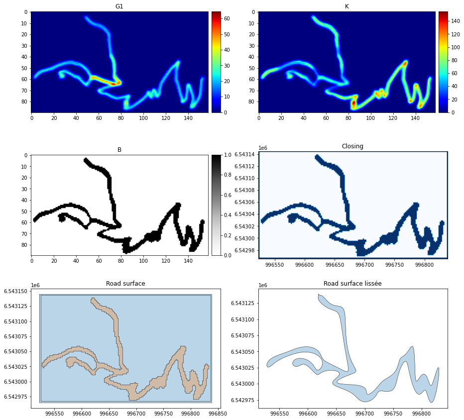
Step 2 : calculs des cartes de densités, de constraste et binaire#
[7]:
from footprint2graph import density_polygonize

# Définition des grilles géométrique et contraste
G1_SIZE              = 2
G2_SIZE              = 30

SEUIL_DENSITE = 25    # pas d'unité
SEUIL_SURFACE = 1000  # m2

cut_factor  = 5

interp_dist = 5
clean_dist  = 0

density_polygonize(RESPATH, G1_SIZE, G2_SIZE, SEUIL_DENSITE, SEUIL_SURFACE,
                       pipeline_idx, cut_factor=cut_factor, interp_dist=interp_dist, clean_dist=clean_dist)
Starting rasterization and vectorization (iteration 1)

    Loading tracks from :  resample_grid
    Number of tracks to load:  877
    Building high-resolution geometry density grid G1 :  2 m ...
    Building low-resolution contextual density grid G2 :  30 m ...
    Assigning track points to the G1 and G2 grids
         500 / 877
    Computing G1 ...
    Computing G2 ...
    Number of neighboring cells to consider: 7
    Building contrast grid :  2 m
    Execution time (seconds): 6.8887412548065186
    Finished heatmap computation.
    Starting morphological closing image ...
100% (291 of 291) |######################| Elapsed Time: 0:00:00 Time:  0:00:00
100% (287 of 287) |######################| Elapsed Time: 0:00:00 Time:  0:00:00
100% (1417 of 1417) |####################| Elapsed Time: 0:00:00 Time:  0:00:00
    Execution time (seconds): 0.23677825927734375
    Finished morphological opening.
Vectorizing cleaned image ...
Extracting road surface vector features ...
    Number of polygonize features:  3
    Number of polygonize features copied:  2
    Execution time (seconds): 0.020345687866210938
    Vectorization completed.
Smoothing polygon to remove stair-step artifacts ...
    Execution time (seconds): 0.07509517669677734
    Road surface smoothing completed.
    Starting centerline computation ...
    Execution time (seconds): 0.18407940864562988
    Centerline computed.
Stage 2 completed: rasterization and vectorization.
[8]:
from footprint2graph.util.PlotRes import plotAFMap, matPlotShapefile, maPlotRasterTiff


plt.figure(figsize=(15, 15))

# ----------------------------------------------------------------------------------------------------------
ax1 = plt.subplot2grid((3, 2), (0, 0))
rasterG1 = tkl.RasterReader.readFromAscFile(RESPATH + 'image/G1_1.asc', name='G1', separator='\t')
mapDensity = rasterG1.getAFMap('G1')
plotAFMap(mapDensity, append=ax1, cmap='jet', vmin=0)

ax2 = plt.subplot2grid((3, 2), (0, 1))
rasterK = tkl.RasterReader.readFromAscFile(RESPATH + 'image/K_1.asc', name='K', separator='\t')
mapContraste = rasterK.getAFMap('K')
plotAFMap(mapContraste, append=ax2, cmap='jet', vmin=0)

# ----------------------------------------------------------------------------------------------------------
ax3 = plt.subplot2grid((3, 2), (1, 0))
rasterB = tkl.RasterReader.readFromAscFile(RESPATH + 'image/B_1.asc', name='B', separator='\t')
mapBinaire = rasterB.getAFMap('B')
plotAFMap(mapBinaire, append=ax3, cmap='Greys', vmin=0)

ax4 = plt.subplot2grid((3, 2), (1, 1))
maPlotRasterTiff(RESPATH, 'image/erosion_1.tif', ax4)
ax4.set_title('Closing')

# ----------------------------------------------------------------------------------------------------------
ax5 = plt.subplot2grid((3, 2), (2, 0))
matPlotShapefile(RESPATH, 'image/road_surface_1.shp', ax5)
ax5.set_title('Road surface')

ax6 = plt.subplot2grid((3, 2), (2, 1))
matPlotShapefile(RESPATH, 'image/road_surface_lissee_1.shp', ax6)
ax6.set_title('Road surface lissée')
[8]:
Text(0.5, 1.0, 'Road surface lissée')
[9]:
report_file(RESPATH, 'image1.json')
=================================================================
                  PIPELINE REPORT INFORMATION

Résultats des calculs matriciels
    Itération n° : 1
    Fin du traitement : 15/06/2026 22:38:55

Image Processing Results
--------------------------------------------------
High-resolution grid cell size :                      2 m
Low-resolution grid cell size :                       30 m
Number of neighboring cells to consider :             7
Cell cluster size threshold for filling or removal :  17 m2

Polygonization Results
--------------------------------------------------
Number of polygonize features :                      3
Number of small polygonized features :               0
Average area of small polygons :                     0 m2
Number of polygonized features above threshold :     2

--------------------------------------------------
Number of edges in the skeleton :      1
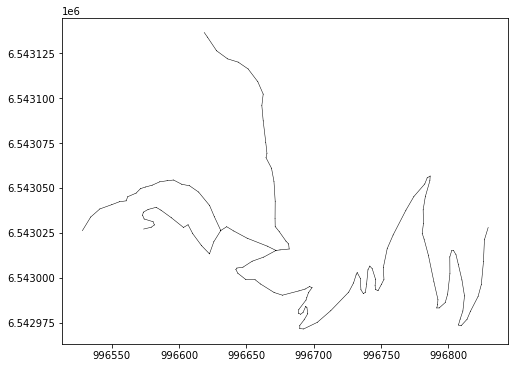
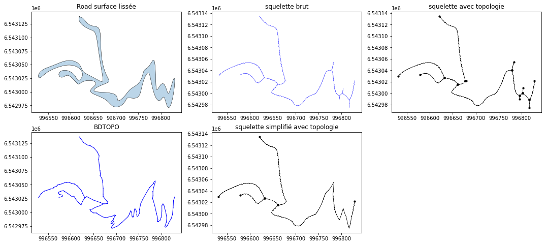
Step 3 : création de la center line#
[10]:
from footprint2graph import addTopologyToNetwork

SEARCH = 25
h = 5
addTopologyToNetwork(RESPATH, SEARCH, h, NB_OBS_MIN, RESAMPLE_SIZE_FUSION, pipeline_idx)

fmt = tkl.NetworkFormat({
           "pos_edge_id": 0,
           "pos_source": 1,
           "pos_target": 2,
           "pos_wkt": 4,
           "srid": "ENU",
           "separator": ",",
           "header": 1})

networkpath = RESPATH + 'network/reseau_1.csv'
squelette = tkl.NetworkReader.readFromFile(networkpath, fmt, verbose=False)
100% (16 of 16) |########################| Elapsed Time: 0:00:00 Time:  0:00:000:00
100% (16 of 16) |########################| Elapsed Time: 0:00:00 Time:  0:00:00
Starting topology creation for the network
    Number of edges in the skeleton: 279
    Finished loaded skeleton.
    /home/md_vandamme/7_LIB/footprint2graph/test/resultjn/network/tmp_in.csv not exists
    /home/md_vandamme/7_LIB/footprint2graph/test/resultjn/network/tmp_out.csv not exists

    Finished removing hooked parts of the skeleton.
    Finished simplification of the skeleton.
Building [100 x 53] spatial index...
    Number of edges in the skeleton (after snapping): 16
    Edge count difference after snapping :  0
    Number of edges in the simplified skeleton: 15
    Number of nodes: 16
     Shortest edges limit :  50
    Number of edges in the skeleton (after removing the shortest edges): 0
    Conflation cannot be performed for node  11 ; the three incident edges are too long: 33 167 284
    Conflation cannot be performed for node  0 ; the three incident edges are too long: 33 64 122
    Edge count after conflation: 5
Stage 3 completed: adding topology to the skeleton.
[11]:
from footprint2graph.util.PlotRes import plotSqueletteTopo, matPlotShapefile

plt.figure(figsize=(18, 8))

ax1 = plt.subplot2grid((2, 3), (0, 0))
matPlotShapefile(RESPATH, 'image/road_surface_lissee_1.shp', ax1)
ax1.set_title('Road surface lissée')

ax2 = plt.subplot2grid((2, 3), (0, 1))
matPlotShapefile(RESPATH + 'network/', 'squelette_1.shp', ax2)
ax2.set_title('squelette brut')

ax3 = plt.subplot2grid((2, 3), (0, 2))
plotSqueletteTopo(RESPATH, ax3)
ax3.set_title('squelette avec topologie')

ax4 = plt.subplot2grid((2, 3), (1, 0))
network.plot(edges='b-', size=1.0, append=ax4)
ax4.set_title('BDTOPO')

ax5 = plt.subplot2grid((2, 3), (1, 1))
squelette.plot('k-', nodes='ko', size=0.8, append=ax5)
ax5.set_title('squelette simplifié avec topologie')

print ('')
[12]:
report_file(RESPATH, 'topology1.json')
=================================================================
                  PIPELINE REPORT INFORMATION

Topologie
    Itération n° : 1
    Fin du traitement : 15/06/2026 22:38:57

--------------------------------------------------
Number of edges in the skeleton :      279
Number of skeleton edges removed for being too short :  0
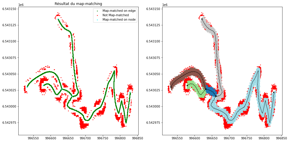
Step 4 : Construction des géométries agrégées pour chaque arc du squelette#
Attribue les points des traces brutes à chaque arc de la topologie
Recalage avec l’algorithme de Newson and Krumm (2009)
Reconstruit les bons morceaux de traces candidats pour chaque arc de la topologie
Agrégation des morceaux de traces
Conflation des traces fusionnées afin d’obtenir un réseau de mobilité
[13]:
from footprint2graph import createNetworkGeom

SEARCH = 25
BUFFER = 20
createNetworkGeom(RESPATH, SEARCH, BUFFER, pipeline_idx)
Starting map-matching, aggregation, and conflation of GNSS trajectories.
    Loading network (1) ...
        Number of edges =  5
        Number of nodes =  6
        Total segment length of the network =  765.9881721625045
    Loading collection of tracks ...
100% (6 of 6) |##########################| Elapsed Time: 0:00:00 Time: 0:00:00
        Number of tracks: 877
        Execution time (seconds): 0.6144757270812988
    Starting map-matching ...
        Index spatial :  [100 x 53] spatial index centered on [996680.2867880978; 6543054.718881102]
Map-matching preparation...
        Parameter search_radius:  25
        Map-matching ended.
        Execution time (seconds): 13.260647058486938
        Prepare map-matching results for candidate segment generation
    Number of map-matched points = 49111 (89.82 %)
    Map-matching results restructuring completed.
        Map-matching results exported.
Starting construction of candidate trajectory segments for each topology edge ...
    265  candidates for edge 15
    571  candidates for edge 12
    264  candidates for edge 16
    189  candidates for edge 17
    235  candidates for edge 21
    Number of processed edges:  5
    Minimum number of candidate tracks per edge:  189
    Maximum number of candidate traces per edge:  571
    Average number of candidate tracks per edge:  305
    Segment construction completed.
        Execution time (seconds): 4.8302083015441895
    Starting track segment aggregation for all network edges ...
        Number of candidate tracks / number of sampled tracks 265 / 30
        Number of candidate tracks / number of sampled tracks 569 / 30
        Number of candidate tracks / number of sampled tracks 264 / 30
        Number of candidate tracks / number of sampled tracks 189 / 30
        Number of candidate tracks / number of sampled tracks 235 / 30
        Number of aggregations: 5
        Number of aggregations with 30 traces: 5
        Number of aggregations with fewer than 30 traces: 0
        Minimum number of traces in aggregation: 189
        Average number of traces in aggregation: 304
        Aggregation process finished.
        Execution time (seconds): 2.6931533813476562
    Starting conflation ...
        Conflation process finished.
        Execution time (seconds): 0.00784158706665039
Stage 4 completed: map-matching, aggregation, and conflation.
[14]:
report_file(RESPATH, 'mapmatch1.json')
=================================================================
                  PIPELINE REPORT INFORMATION

Map Matching
    Itération n° : 1
    Fin du traitement : 15/06/2026 22:39:12

Search radius (m):                25

Results
--------------------------------------------------
Map-matched points:               49111 ( 89.82 % )
Off-track points:                 5564 ( 10.18 % )

Quality
--------------------------------------------------
Root Mean Square Error (RMSE) :   3 m
Maximal displacement :            8.58 m
[15]:
report_file(RESPATH, 'candidate1.json')
=================================================================
                  PIPELINE REPORT INFORMATION

Préparation des traces pour la fusion: segments candidats
    Itération n° : 1
    Fin du traitement : 15/06/2026 22:39:16

Results
--------------------------------------------------
Number of processed edges :                         5
Minimum number of candidate traces per edge :       189
Maximum number of candidate traces per edge :       571
Average number of candidate tracks per edge  :      305
[16]:
report_file(RESPATH, 'aggregate1.json')
=================================================================
                  PIPELINE REPORT INFORMATION

Aggrégation des segments de traces candidats
    Itération n° : 1
    Fin du traitement : 15/06/2026 22:39:19

Results
--------------------------------------------------
Number of aggregations :                            5
Number of aggregations with 30 traces :             5
Number of aggregations with fewer than 30 traces :  0
Minimum number of traces in aggregation :           189
Average number of traces in aggregation :           304
[17]:
report_file(RESPATH, 'conflate1.json')
=================================================================
                  PIPELINE REPORT INFORMATION

Conflation de la géométrie du réseau sur le squelette
    Itération n° : 1
    Fin du traitement : 15/06/2026 22:39:19

Results
--------------------------------------------------
Segments conflated :             5 ( 100.0 % )

Distorsion
--------------------------------------------------
Total distorsion RMSE :          3.268 m
Maximum distorsion RMSE :        16.67 %
Visualisation du recalage sur le réseau#
[18]:
from footprint2graph.util.PlotRes import plotMM

plotMM(RESPATH, squelette)
plt.show()
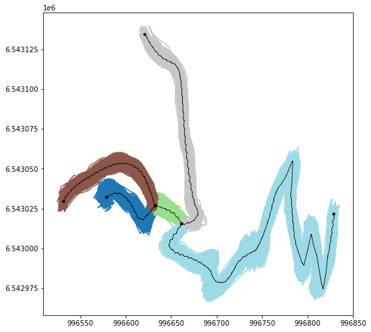
Visualisation des candidats pour l’agrégation#
[19]:
from footprint2graph.util.PlotRes import plotSegmentsConstruction

plt.figure(figsize=(8, 8))

ax1 = plt.subplot2grid((1, 1), (0, 0))
plotSegmentsConstruction(RESPATH, ax1, squelette)
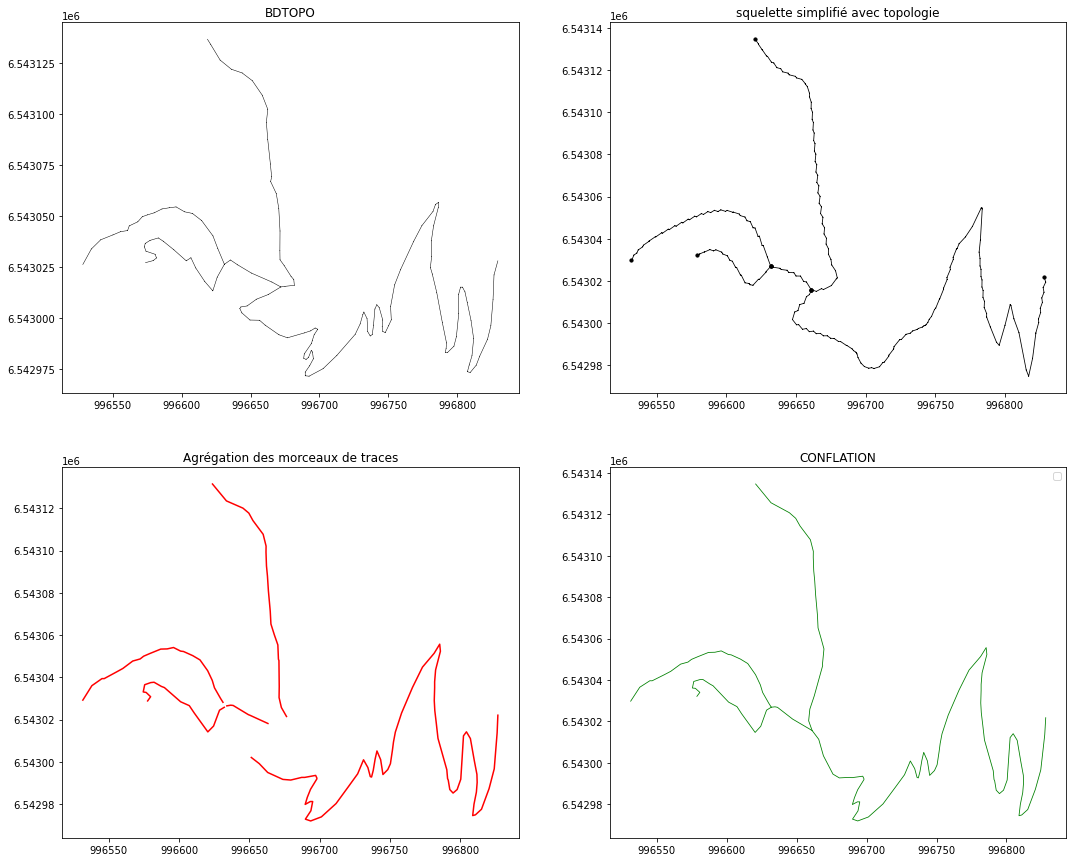
Visualisation de l’agrégation et de la conflation#
[20]:
from footprint2graph.util.PlotRes import plotAggregation, plotConflation
import os

plt.figure(figsize=(18, 15))

# ---------------------------------------------------
ax1 = plt.subplot2grid((2, 2), (0, 0))
network.plot('k-', '', 'g-', 'r-', 0.5, ax1)
ax1.set_title('BDTOPO')

# ---------------------------------------------------
ax2 = plt.subplot2grid((2, 2), (0, 1))
squelette.plot('k-', nodes='ko', size=0.8, append=ax2)
ax2.set_title('squelette simplifié avec topologie')

# ---------------------------------------------------
ax3 = plt.subplot2grid((2, 2), (1, 0))
plotAggregation(RESPATH, ax3)
ax3.set_title('Agrégation des morceaux de traces')

# ---------------------------------------------------
ax4 = plt.subplot2grid((2, 2), (1, 1))
plotConflation(RESPATH, ax4)
ax4.set_title('CONFLATION')
[20]:
Text(0.5, 1.0, 'CONFLATION')
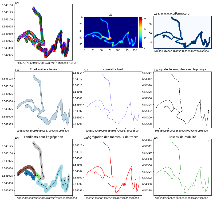
Regards sur le pipeline de construction#
[21]:
plt.figure(figsize=(15, 15))

# ---------------------------------------------------
ax1 = plt.subplot2grid((3, 3), (0, 0))
collection.plot(append=ax1)

ax2 = plt.subplot2grid((3, 3), (0, 1))
rasterG1 = tkl.RasterReader.readFromAscFile(RESPATH + 'image/G1_1.asc', name='G1', separator='\t')
mapDensity = rasterG1.getAFMap('G1')
plotAFMap(mapDensity, append=ax2, cmap='jet', vmin=0)

ax3 = plt.subplot2grid((3, 3), (0, 2))
maPlotRasterTiff(RESPATH, 'image/erosion_1.tif', ax3)
ax3.set_title('Fermeture')

# ---------------------------------------------------
ax4 = plt.subplot2grid((3, 3), (1, 0))
matPlotShapefile(RESPATH, 'image/road_surface_lissee_1.shp', ax4)
ax4.set_title('Road surface lissée')

ax5 = plt.subplot2grid((3, 3), (1, 1))
matPlotShapefile(RESPATH + 'network/', 'squelette_1.shp', ax5)
ax5.set_title('squelette brut')

ax6 = plt.subplot2grid((3, 3), (1, 2))
squelette.plot('k-', nodes='ko', size=0.8, append=ax5)
ax6.set_title('squelette simplifié avec topologie')

# ---------------------------------------------------
ax7 = plt.subplot2grid((3, 3), (2, 0))
plotSegmentsConstruction(RESPATH, ax7, squelette)
ax7.set_title("candidats pour l'agrégation")

ax8 = plt.subplot2grid((3, 3), (2, 1))
plotAggregation(RESPATH, ax8)
ax8.set_title('Agrégation des morceaux de traces')

ax9 = plt.subplot2grid((3, 3), (2, 2))
plotConflation(RESPATH, ax9)
ax9.set_title('Réseau de mobilité')
[21]:
Text(0.5, 1.0, 'Réseau de mobilité')